Sizing LLM inference without a GPU run
Every team putting an LLM into production faces the same expensive question: how many GPUs, configured how, for the traffic pattern they expect to serve?
Today, teams benchmark a handful of configurations and extrapolate from a space of tens of thousands. We take a different approach: we simulate the serving stack, run through every permutation and combination of the configuration in under ten minutes, and find the optimal deployment configuration before running a single GPU experiment.
This post explains how you get to the optimal GPU deployment configuration fast, and how close the predictions land to real hardware.
01How many GPUs?
Say you’re about to put a 27-billion-parameter model into production. You need it to serve, say, 5,000 tokens a second to your users, and your traffic looks like a coding assistant: ISL ~8,000 tokens, OSL ~300. Then we have to answer: how many H100s do we rent, and how do we run them?
This is not division. Dividing required throughput by single-GPU throughput assumes per-GPU throughput is a constant, and it is not: it depends on how you split the model and on the traffic you serve. The same eight H100s deliver 1,255 or 2,325 tok/s depending only on how the model is split across them, and adding GPUs returns less than linear throughput.
On-demand, an 8×H100 node runs between $55.04 and $98.32 an hour depending on the provider. Every cost in this post is priced at $50/hr - a round figure below the cheapest of those, so the numbers here understate what you would actually pay. Even at that rate one node is $438,000 a year, used or idle.
Buy too many and the waste is obvious - provision 64 GPUs where 24 would have carried the load and you’re paying for 40 idle cards, month after month. Under-provisioning costs more than the GPUs you skipped: you miss your latency target, requests queue, and users see a laggy product. And the fix is slow - adding GPUs means new hardware, re-testing the configuration, and redeploying, so a shortfall you find in production can take weeks to close.
The third failure mode is the least obvious: you can buy the right number of GPUs and still throw away half your performance by arranging them wrong. Eight GPUs can run as one replica split across all eight, as eight independent single-GPU replicas, or several ways in between. In our tests two configurations of the same eight cards delivered 1,255 versus 2,325 tok/s - nearly double, from identical hardware, at essentially the same per-token latency. And no configuration wins for every workload, so the answer you buy today can be wrong in six months.
Figure 1 recasts those numbers as unit cost - the hourly rate of the nodes a configuration occupies, over the output tokens it actually produces in that hour:
\[ \text{cost per Mtok} \;=\; \frac{\text{node rate }(\$/\text{hr})}{\text{tok/s}\;\times\;3600 \;/\; 10^{6}} \]
At $50/hr per 8-GPU node, 1,255 tok/s gives \(\$50 / 4.518 = \$11.07\) per million output tokens. Every point is measured.
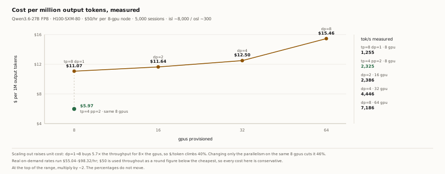
dp=1 to dp=8 buys 5.7× the throughput for 8× the GPUs, so cost per million output tokens climbs 40%, from $11.07 to $15.46. And on a fixed 8 GPUs, changing only the parallelism to tp=4/pp=2 cuts unit cost 46% to $5.97, cheaper than every scaled-out option here. Real on-demand rates for this node run $55.04-$98.32/hr, so at the top of that range multiply every figure by about two - the percentages do not move, because they are ratios. The sizing question is therefore not only how many GPUs, but which configuration you run on them.02Why the answer depends on your traffic
Every request runs two phases with different bottlenecks. Prefill processes the whole prompt in one forward pass and saturates the GPU’s arithmetic units, so it is compute-bound. Decode emits one token per iteration, and every iteration re-reads the KV cache of every request in the batch. Arithmetic per token is negligible, so decode is bound by memory bandwidth: the rate the GPU streams the KV cache out of HBM.
Every quantity used in this post, defined once:
| Term | Definition | Unit |
|---|---|---|
| TTFT | Time to first token, measured from request submission, so it includes queueing | ms |
| TPOT | Time per output token, averaged over a request’s decode tokens | ms |
| Decode throughput | Output tokens per second summed over all in-flight requests | tok/s |
| Concurrency | Requests in flight at once, admitted and not yet finished | requests |
max_num_batched_tokensthe “token budget” | Most tokens the scheduler may place in one forward pass, across the whole batch. Not a per-request sequence limit | tokens |
| KV cache capacity | HBM bytes available for the paged KV cache after weights and margin | bytes |
| Memory bandwidth | Rate the GPU streams KV cache and weights out of HBM | bytes/s |
| ISL / OSL | Input and output sequence length per request | tokens |
Which limit binds first depends on traffic shape:
- A coding assistant sends huge prompts - the whole file, the repo context - and gets short edits back. At ISL ~8,000 and OSL ~300, prefill is 96% of the token work. What binds is the token budget: a prompt larger than one forward pass can hold is admitted in chunks, one chunk per iteration - 2 chunks at a 6,144-token budget, 12 at 682. Each of those iterations spends most of its budget on prefill and has little left for decode, so decode tokens per iteration drop and aggregate decode throughput falls for the whole batch while that prompt is being read. Every request already decoding waits longer for its next token, so TPOT rises for all of them. The chunked request needs 12 iterations before its first output token instead of 2, so its TTFT rises with the chunk count.
- A chatbot sends short prompts and needs a steady stream of words back. Prefill is over quickly, so the request is almost entirely decode, and one iteration advances every active request by exactly one token - so TPOT is iteration time. Admitting one more request lengthens that iteration, because the GPU must compute one more token and stream one more request’s KV cache through HBM within the same forward pass. With a 50 ms per-token SLO against the ~48 ms p99 TPOT measured for this model on an H100 node, 2 ms of margin remain: the next admission consumes it and the one after breaches the SLO. So the SLO caps batch size, and because throughput scales with batch size it caps tokens per second per GPU. Serving the same traffic then takes more replicas - you buy GPUs to hold a latency line rather than to do work. Memory is not the constraint here: each request holds ~125 MB of KV cache, so 72 GB would hold roughly 590 concurrent requests, far more than the latency target allows.
- A reasoning or agent workload writes far more than it reads - long chains of thought, thousands of output tokens. Every one appends to the KV cache, so a request that begins with 2,000 tokens of cache ends holding 12,000: 250 MB becomes 1.5 GB. Capacity: the same 72 GB holds 295 of these requests at the start but 49 once grown, so as the live requests age fewer new ones fit, the batch drains faster than it refills, and aggregate throughput decays over the run. Bandwidth: decode re-reads the entire live cache every iteration, so bytes streamed per iteration grow as the caches grow and TPOT rises as requests age.
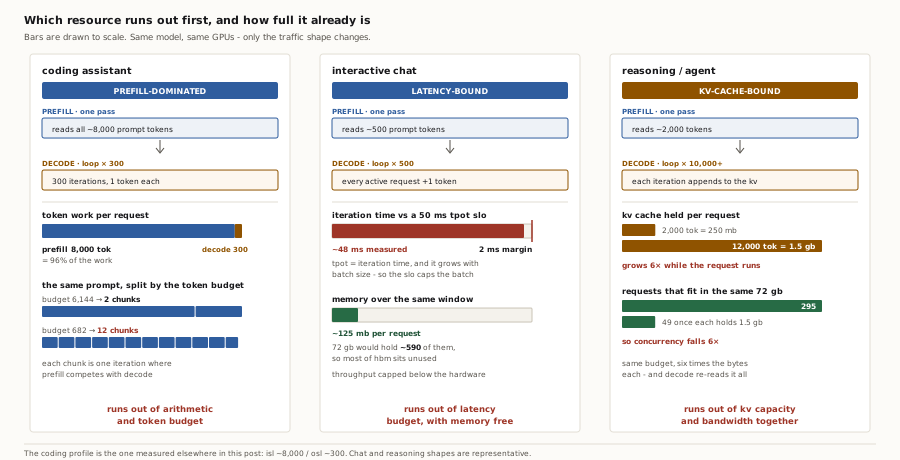
A benchmark published for one of these traffic shapes carries no information about the others.
The knobs that decide it
Each knob trades one outcome against another. The direction, the mechanism, and where the direction stops holding:
- Tensor parallelism,
tensor_parallel_size. Each GPU holds a shard of every layer, so weight bytes, KV-cache bytes and arithmetic per GPU per token all fall roughly as 1/TP - and because decode is bandwidth-bound, less to stream means a shorter step. That benefit has a ceiling. Two all-reduces run per layer, one after attention and one after the MLP; the bytes each GPU sends level off as TP grows, but the number of synchronisation steps does not, and the cost jumps whenever the group stops fitting inside one fast interconnect domain. KV sharding also stops at the model’s KV-head count. Meanwhile total GPUs = tensor parallelism × pipeline parallelism × replicas, so at a fixed GPU count raising TP costs you replicas. Figure 3 shows TP=8 sitting past the useful point for this model: against TP=4 with PP=2 on the same 8 GPUs it delivers 46% less throughput, at 48 ms p99 TPOT against 47 ms - no latency gain at all. That comparison moves PP as well, so it bounds the benefit of higher TP rather than isolating it - but it is enough to say there is no single direction here. TP has a useful range, and 8 is above it. - Replicas,
data_parallel_size. Each replica is a full copy of the model with its own GPUs, so aggregate throughput rises with replica count - sublinearly, and only while arrivals keep every replica batched. Nothing pools across replicas: weights are duplicated per replica, the prefix cache is per-replica so a 70% hit rate inside one replica does not become 70% across eight, and a request routed to a busy replica cannot borrow a quiet one’s free KV blocks. In Figure 3,dp=1todp=8gives 5.7×, not 8×. Every configuration in that sweep is backlogged - average TTFT is 117 seconds even atdp=8- so it is a saturated-throughput comparison rather than a latency one, and the gap against linear scaling is not attributable to any single one of those causes from this data alone. - Batch size, capped by the token budget, by
max_num_seqs, and by free KV blocks - whichever binds first. Larger batches raise decode throughput because the weight bytes streamed per iteration are amortised across more tokens. While weight bytes dominate, step time is nearly flat as the batch grows, so that throughput is close to free. It stops being free in two ways. Once the live KV cache outweighs the weights - the reasoning case above, at 1.5 GB per request - every added request adds bytes to stream and step time grows with batch size directly. And once kernels turn compute-bound, step time grows with arithmetic instead. Either way TPOT is what pays. Net: throughput up, TPOT up, cheap only in the weight-dominated regime. - Precision and KV-cache format. FP8 weights instead of BF16 halve weight bytes, which frees HBM for KV cache and cuts what decode must stream, relieving capacity and bandwidth together. An FP8 KV cache does the same to the cache itself. What it costs is output quality, and not equally: quantising the KV cache degrades more than quantising weights at the same width, because the cache is read back as attention state for the rest of the request. Kernel support also varies by GPU, so the gain does not carry across the hardware axis of the grid.
The knobs are coupled, which is why they cannot be tuned one at a time: tensor parallelism changes how many replicas fit, batch size moves you between bandwidth-bound and compute-bound, and precision moves the capacity and bandwidth limits together while changing output quality.
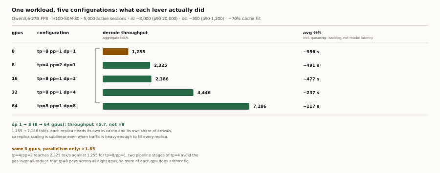
dp=1 to dp=8 - 8 GPUs to 64 - multiplies decode throughput by 5.7, not 8. On a fixed 8 GPUs, changing only the parallelism to tp=4/pp=2 gives 1.85×. TTFT here is dominated by queueing at 5,000 arrivals, so read the fall from ~956 s to ~117 s as backlog draining, not as model latency.03Why you can’t just test every option
The obvious answer is to measure. Set up each option, send it realistic traffic, write down how fast it runs, and pick the best. Testing like this works, and it should always be the final check before you commit. The problem is that there are far too many combinations to test them all.
A meaningful benchmark run - enough traffic to reach steady state and read a stable number - takes roughly 30 minutes on the GPUs the configuration needs. At $50/hr for an 8×H100 node, a single 8-GPU test costs about $25. Test 50 configurations and you’re at about $1,250 and a full day of machine time; do it properly - a few traffic levels each, repeated for noise - and it’s closer to $6,000 and a week.
Now count the configurations. Each of these is a real choice you have to make, and they multiply:
| Parameter | Typical options | Count |
|---|---|---|
| GPU type | A40, A100, H100, H200 | 4 |
| Tensor parallelism | 1, 2, 4, 8 | 4 |
| Pipeline parallelism | 1, 2, 4 | 3 |
| Replicas | 1 up to the node count | 4 |
| Precision | FP8, BF16, INT8… | 3 |
| KV-cache format | FP16, FP8 | 2 |
| max_num_batched_tokens | a handful of settings | 5 |
| Serving mode | co-located, disaggregated | 2 |
| Multiplied together | 11,520 | |
And that is a conservative slice - it leaves out finer scheduler and runtime knobs. Figure 4 takes this exact grid through the pipeline. At $25 a test, running even this reduced grid on real hardware would cost around $290,000 and take months. In practice teams test a handful of configurations, pick the least-bad one, and leave most of the space unexplored.
As your product grows, prompts get longer, traffic rises, and usage patterns shift - and the configuration that won at launch may not win six months later. You can’t spend $6,000 and a week every single time your traffic changes.
04How we search the whole space
The whole search runs on CPUs. No GPU is touched while we explore the 11,520 configurations - we simulate each one. The most detailed simulator replays the serving engine’s scheduler step by step, and even at a few seconds per configuration that would still take hours across the full grid. So we don’t run the detailed simulator on everything.
Instead we filter in stages, cheapest first. The early stages are nearly free and run on every configuration, dropping the ones that can’t work. Only the 20 selected candidates reach the detailed simulation. The early stages are set algebra over model and device facts, so they are orders of magnitude cheaper per candidate than a scheduler replay; we report the candidate counts each stage admits and rejects, not per-stage timings.
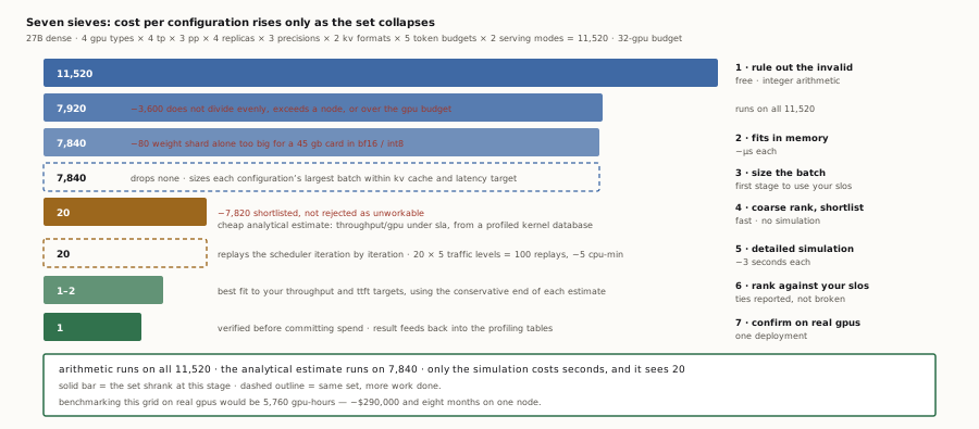
The search is a sieve of seven stages, cheapest first. Each stage runs on everything the previous one passed, and each costs more per configuration than the last while seeing far fewer of them. The counts below are for the 11,520-configuration grid in the table above.
- Rule out the invalid. Tensor parallelism has to divide both the attention head count and the embedding width, pipeline depth has to divide the layer count, the configuration has to fit inside one node, and GPUs per replica times replica count has to stay within the GPU budget you are willing to provision. Integer arithmetic on the model shape, so effectively free. Removes 3,600 of 11,520, leaving 7,920. One consequence surfaces later: when tensor parallelism exceeds the number of key/value heads, those heads are replicated rather than split, so past that point the KV cache stops shrinking as you add GPUs.
- Check it fits in memory. Per GPU, take 90% of the card as the budget, subtract the weight shard, and convert what remains into fixed 16-token KV cache pages. Reject anything whose weights alone overflow the budget, or that cannot hold one page plus a 1% reserve. Microseconds. Removes 80, leaving 7,840 - all of them a 45 GB card trying to hold a 27B model in BF16 or INT8. On 80 GB cards nothing fails here, which is itself worth knowing.
- Size the batch. For each surviving configuration, sweep batch size and parallelism to find the largest batch it can actually run before it either runs out of KV cache or misses your latency target. This is the first stage that consults your SLOs rather than just the hardware, and it is why a configuration that looks feasible on memory alone can still turn out useless.
- Coarse rank, and shortlist. A cheap analytical estimate - throughput per GPU under your SLA, read from a profiled kernel database with interpolation rather than by simulating anything - orders what is left and keeps the top 20, with a limit of three sharing the same GPU model and parallelism shape so one family cannot take every slot. This is the decisive cut: 7,840 down to 20. It is fast enough to run on everything, which is the whole reason it comes before the simulator.
- Detailed simulation. Now, and only now, the event simulator runs on the survivors. It replays the serving engine’s scheduler iteration by iteration - admission, the per-iteration token budget, chunked prefill - reading each operation’s time from the profiled table. About 3 seconds per configuration on CPU. Twenty configurations across five traffic levels is 100 replays, minutes of CPU time.
- Rank against your SLOs. Configurations are scored on how well they fit the targets you actually gave - throughput and time-to-first-token - using the conservative end of each simulated estimate rather than the midpoint. A configuration whose conservative bound clears your target is reported differently from one that only clears it on the point estimate, and when two cannot be separated we say so instead of inventing a winner.
- Confirm on real hardware. The one or two finalists get a real deployment on real GPUs to verify the number before you commit the spend. That run also feeds back into the profiling and calibration data, so the next search starts from better tables.
The shape of the cost is the point. Stages 1 and 2 are arithmetic and run on all 11,520. Stages 3 and 4 are analytical estimates, cheap enough to run on everything that survived. Only stage 5 costs seconds, and it sees 20. Only stage 7 touches a GPU, and it sees one. Set against the alternative: benchmarking the full grid on real GPUs is 5,760 GPU-hours, about $290,000 and eight months on a single node. This path is a CPU search measured in minutes, plus one confirmation run on GPUs - $25 of hardware.
Why being within 8% is good enough
Assumption: candidate decode throughputs are separated by more than the prediction error. Ranking does not need exact speeds, only correct order. An 8% band preserves the order whenever candidates differ by more than that; when two fall inside it we report a tie and name the single benchmark that settles it. Benchmarking is not removed, it is reduced to the one or two configurations where it changes the decision.
05The prediction holds on real hardware
We served Qwen 3.6 27B FP8 with vLLM on H100s at TP=2, drove it with SWE-bench coding traces, and compared predicted against measured decode throughput in every two-minute window, with nothing trimmed and no outliers removed.
max_num_batched_tokens is the per-iteration token budget: the most tokens the scheduler may place in one forward pass across every request in the batch. It is not a per-request sequence limit. Dividing it by concurrency gives the tokens available per in-flight request, which is the quantity the error tracks.
| Concurrency | max_num_batched_tokens | Tokens per request | Measured | Predicted | Error |
|---|---|---|---|---|---|
| 8 | 49,152 | 6,144 | 107.6 tok/s | 107.7 tok/s | +0.10% |
| 14 | 32,768 | 2,341 | 123.6 tok/s | 113.5 tok/s | −8.20% |
| 12 | 8,192 | 683 | 114.2 tok/s | 104.3 tok/s | −8.70% |
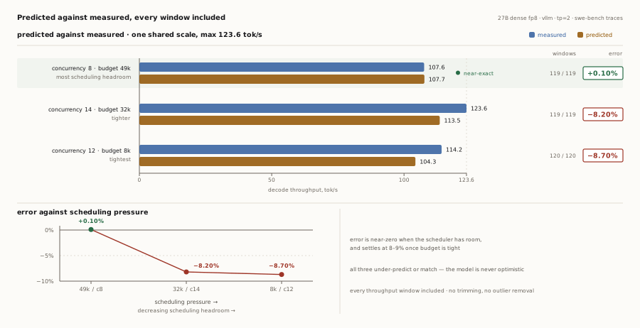
Across every configuration tested, predicted decode throughput lands within 8.7% of measured. Two things about how that error behaves matter more than the headline figure: what it tracks, and which direction it points.
The error tracks the per-request token budget, not concurrency. With 6,144 tokens available per request the prediction lands within 0.10%; at 2,340 and 682 tokens per request it under-predicts by about 8%.
Prompt chunking explains it. An 8,000-token prompt cannot enter a single forward pass unless the per-request budget covers all 8,000, so the scheduler splits it into chunks and feeds one chunk per iteration. At 6,144 tokens per request the prompt is split into 2 chunks and so occupies 2 iterations. At 682 tokens per request the same prompt is split into 12 chunks and occupies 12 iterations. In every one of those iterations the prefill chunk competes with decode work for the same token budget, and that contention is the part the prediction models least well - which is why the tighter budgets carry the 8% error.
Concurrency does not explain the ordering: the middle row runs at higher concurrency than the last.
The direction is consistent: all but one comparison under-predicts, and the exception over-predicts by 0.10%. For sizing that is the safe direction - if we say a configuration sustains 5,000 tok/s and we under-predict, the real hardware has slightly more headroom than promised, not less.
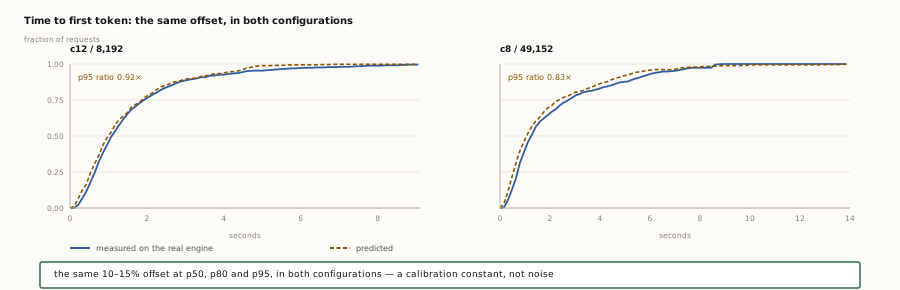
The safe direction holds for throughput, not for percentile latency. Aggregate decode throughput we under-predict, so real hardware has more headroom than promised. Predicted p95 time-per-output-token goes the other way - it comes in below measured, which is optimistic, and contention under heavy load is the cause. So treat predicted p95 TPOT as a lower bound: size on throughput, and if you hold a strict p95 latency SLO, make that the number you confirm on hardware before committing.
Windowed tracking, not just the mean
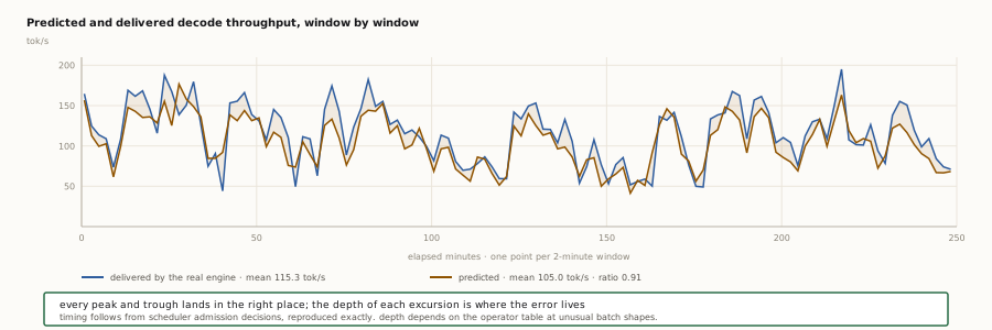
A matching mean can come from cancelling errors, so the stronger test is whether the prediction tracks throughput as traffic rises and falls. Below is the same four-hour run in two-minute windows.
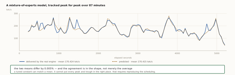
We ran the same test on a mixture-of-experts model, Qwen 3.6 35B-A3B, where per-token compute depends on which experts each token activates - harder to predict. The match was tighter still.
Both sides ran the same work
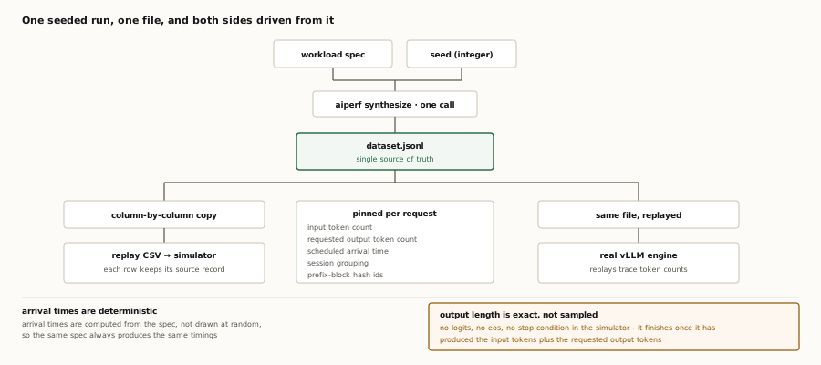
The comparison only means anything if the simulator and the real engine were handed identical work. They were - not because we compared two graphs afterwards and found them similar, but because there is only ever one trace.
AIPerf generates it once, from a fixed seed, using its agentic code-generation dataset. That is why the traffic looks like a coding assistant. AIPerf then validates its own output. That single file is the only source of truth: the CSV the simulator reads is a column-by-column copy of it, and every row still carries the original record it came from, so any individual request can be checked against the source rather than trusted because a histogram matched.
Arrival times are deterministic: each request sits at a fixed point in the schedule rather than being drawn at random, so the same spec always produces the same timings. Five fields are pinned per request - input length, requested output length, arrival time, which session it belongs to, and the prefix blocks that decide cache reuse. Output length is exact on the simulator side because there is no sampler in it at all: no logits, no end-of-sequence token, nothing that could stop early. It counts, and a request finishes once it has produced its input tokens plus the output tokens the trace asked for. One precondition belongs in the run config rather than the data: replay can scale token counts and can trim prompts longer than the configured maximum, so this holds only when those scale factors are 1.0 and the maximum exceeds the longest request in the trace.
The system predicts throughput accurately enough to get the full ranking right. It tells you which configurations are clearly better, flags the handful that are genuinely too close to call, and sends only those few to real hardware to settle. That is what sizing needs: approximate SLO numbers for every configuration - throughput and latency estimated closely enough to order the candidates and to say which ones are worth measuring - rather than an exact speed for any single one of them.
06Where the accuracy comes from
Decode throughput is output tokens over wall-clock time. We decompose that into three segments, each modelled and validated on its own:
- Iteration cost. For a fixed batch, what is the wall-clock time of one forward pass? This is where the hardware lives: bytes streamed over weights and KV cache against HBM bandwidth, per-operator kernel latency read from a profiled table and interpolated across shapes, collective cost (all-reduce, send/recv) profiled per node topology, and attention-family-specific KV cache memory layouts for GQA, MQA, MLA and sliding-window.
- Batch composition. Which requests occupy that pass? This is scheduler policy rather than hardware: admission against the per-iteration token budget, chunked prefill splitting long prompts across steps, preemption and rollback when KV blocks run short, prefix-cache hits shortening prefill, and paged block allocation. It does not collapse into an average batch size or a utilisation factor, which is why we replay the scheduler instead of approximating it.
- Arrival process. What drives the two above? Request count, ISL and OSL distributions, inter-arrival timing, session structure and prefix-reuse pattern - taken from the materialised trace rather than modelled.
Compose them - iteration cost over the batch the scheduler assembled, driven by the arrival process - and you have throughput. Validating each segment separately is what makes a miss diagnosable instead of mysterious.
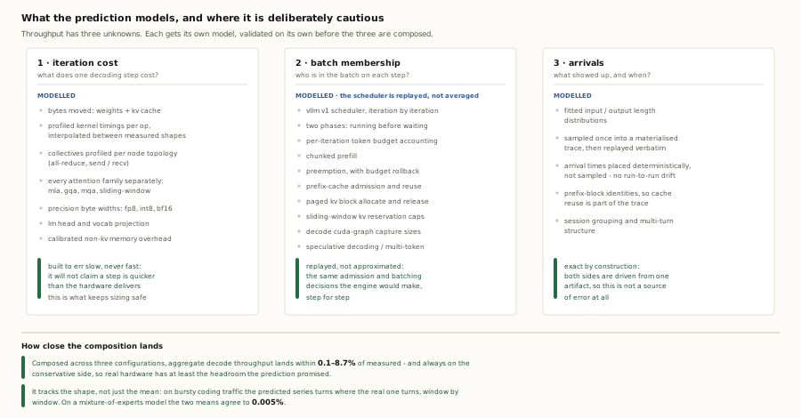
Two of these carry most of the risk. Iteration cost: We combine hardware limits with measured kernel behaviour, and the model is deliberately biased slow rather than fast: it will not claim a step is quicker than the hardware delivers. That is why the throughput number stays conservative. And the scheduler: which requests share a batch, when prompts are admitted, how prefill competes with decode. That cannot be reduced to an average batch size, so we replay the real vLLM scheduler instead.
07Three workloads, three different answers
We ran three traffic patterns through the search on the same model and GPU fleet. Each returned a different best configuration, because each binds on a different limit.
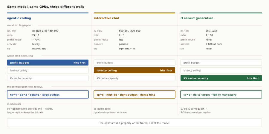
The best configuration can change with load alone: one that wins at one level of concurrent in-flight requests can fall behind a different one when that load rises only slightly, because the extra requests tip it past a KV cache capacity or latency limit that the other configuration absorbs. Eight replicas give about 5.7× the throughput of one, not 8×, and even that only shows up once there’s enough traffic to keep all eight busy - more replicas raise the throughput ceiling, they do not create traffic. And two configurations of the same 8 GPUs can be nearly 2× apart in throughput at the same latency, purely from how they’re wired. None of this appears on a spec sheet. It emerges only when real traffic competes for the batch, the KV cache, and the GPU, which is what the scheduler replay reproduces.
08Sizing this for your own workload
If you’re staring at the same question - how many GPUs, arranged how, for the traffic you serve today and the traffic you’re growing into - you don’t have to guess your way to an answer or burn weeks of GPU time benchmarking a handful of configurations. Describe your model and the traffic you expect, and we’ll search the space for you and come back with the configuration that fits, the GPU count behind it, and the evidence for why.
Facing this problem? If you’re sizing an LLM deployment and want the right answer before you commit the budget, get in touch - tell us your model and workload, and we’ll help you find the optimal deployment configuration.